Quickstart Guide
You don’t need to know every detail of every method to get CytofDR working. In fact, you don’t even
need to know much Python. CytofDR is a flexible and extensible framework to allow you to perform
and benchmark dimension reduction all in one place with human readable codes. Here, there are examples
to walk you through every step of the way! Scroll to Pipeline At a Glance for TLDR.
Loading Dataset
The first step of the process is loading your CyTOF sample into Python. The CytofDR package uses the
numpy framework extensively, which means that loading expression matrices are fairly easy. Here, we
assume that all your datasets have been preprocessed and only lineage channels are preserved. If you need
to preprocess your data, you can use our sister package PyCytoData.
Assume that you have a csv with the rows as cells and columns as features. Further, the first row is feature names, here is what you can do:
>>> import numpy as np
>>> expression = np.loadtxt(fname="PATH_To_file", dtype=float, skiprows=1, delimiter=",")
Voila, you have an expression matrix in an array! You can view the array by simply calling it:
>>> expression
array([[1.73462413, 2.44479204, 0.        , ..., 0.22536523, 1.02089248, 0.1500314 ],
       [0.56619612, 1.52259608, 0.        , ..., 0.31847633, 0.        , 0.        ],
       [0.54875404, 0.        , 0.        , ..., 0.17807296, 0.46455456, 3.55193468],
       ...,
       [0.1630427 , 0.32121831, 0.        , ..., 0.61940005, 0.        , 3.50253287],
       [0.30990439, 2.59020988, 0.11689489, ..., 0.94090453, 0.1383413 , 0.        ],
       [0.71138557, 1.72764796, 0.        , ..., 0.        , 0.        , 0.        ]])
Note
CytofDR does not support working with fcs files directly!
Note
For outputs, we will use the example of the Oejen cohort Sample U.
Using PyCytoData
PyCytoData is our sister package that specifically handles CyTOF data IO as well as preprocessing.
This allows us to have a consistent interface across multiple different packages, much like the
same engine but with different accessories. Here, we will should you how to load a dataset
with PyCytoData:
>>> from PyCytoData import FileIO

>>> dataset = FileIO.load_expression(files="/path",
...                                  col_names=True,
...                                  delim="\t")
>>> dataset.expression_matrix
array([[1.73462413, 2.44479204, 0.        , ..., 0.22536523, 1.02089248, 0.1500314 ],
       [0.56619612, 1.52259608, 0.        , ..., 0.31847633, 0.        , 0.        ],
       [0.54875404, 0.        , 0.        , ..., 0.17807296, 0.46455456, 3.55193468],
       ...,
       [0.1630427 , 0.32121831, 0.        , ..., 0.61940005, 0.        , 3.50253287],
       [0.30990439, 2.59020988, 0.11689489, ..., 0.94090453, 0.1383413 , 0.        ],
       [0.71138557, 1.72764796, 0.        , ..., 0.        , 0.        , 0.        ]])
Well, this look very similar to the numpy interface. Indeed, you can access the array
just as usual. You can extract the array if you wish, but you can also use this object as
we document in the Working with PyCytoData
section. In fact, PyCytoData is much more interesting than simply just a wrapper for the numpy method.
Dimension Reduction
DR running DR is as easy as copy some code and hitting enter! Let’s say you want to run UMAP, tSNE, and PCA–three of the most popular methods. You can simply do the following:
>>> from CytofDR import dr
>>> results = dr.run_dr_methods(expression, methods=["umap", "open_tsne", "pca"])
Running PCA
Running UMAP
Running open_tsne
===> Finding 90 nearest neighbors using Annoy approximate search using euclidean distance...
--> Time elapsed: 81.40 seconds
===> Calculating affinity matrix...
--> Time elapsed: 2.84 seconds
===> Running optimization with exaggeration=12.00, lr=10243.67 for 250 iterations...
Iteration   50, KL divergence 6.8745, 50 iterations in 2.1659 sec
Iteration  100, KL divergence 6.3337, 50 iterations in 2.2041 sec
Iteration  150, KL divergence 6.2017, 50 iterations in 2.3244 sec
Iteration  200, KL divergence 6.1405, 50 iterations in 2.2421 sec
Iteration  250, KL divergence 6.1041, 50 iterations in 2.2620 sec
--> Time elapsed: 11.20 seconds
===> Running optimization with exaggeration=1.00, lr=10243.67 for 250 iterations...
Iteration   50, KL divergence 4.8511, 50 iterations in 2.1616 sec
Iteration  100, KL divergence 4.3954, 50 iterations in 2.1746 sec
Iteration  150, KL divergence 4.1621, 50 iterations in 2.2973 sec
Iteration  200, KL divergence 4.0129, 50 iterations in 2.5909 sec
Iteration  250, KL divergence 3.9067, 50 iterations in 2.9614 sec
--> Time elapsed: 12.19 seconds
We have some handy printouts to remind you what is running, but if you would like disable so that
it doesn’t clutter your precious console screen, you can specify verbose=False.
Access Embeddings
You can easily access the embeddings of that are stored in the object by accessing the reductions
dictionary and use the method names as keys.
>>> results.reductions["UMAP"]
array([[-1.1084751 , 10.174761  ],
       [ 0.7808647 , -2.341636  ],
       [12.979893  , -5.1433287 ],
       ...,
       [11.690209  , -5.4123435 ],
       [ 0.9842613 , -2.8788142 ],
       [ 1.6086756 , -0.92493653]], dtype=float32)
To know the names of your embeddings, you can simply run
>>> results.names
{'PCA', 'UMAP', 'open_tsne'}
which returns a set.
Plotting Results
One of the main goals of DR is to visualize the data! Wanna know whether T cells are next to B cells? We’ve got your back like your best friend! You can simply run the following:
results.plot_reduction("umap", save_path="PATH_To_FILE")
Here is an example of the embedding:
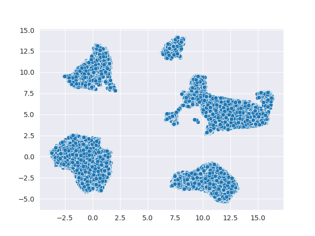
Umm, something is missing! There’re no labels: it looks a bit dull! If you have labels or
cell types, you can do so by specifying the hue parameter:
## ``labels`` is a numpy array of labels
results.plot_reduction("umap", save_path="PATH_To_FILE", hue=labels)
Here are the results of colored clusters:
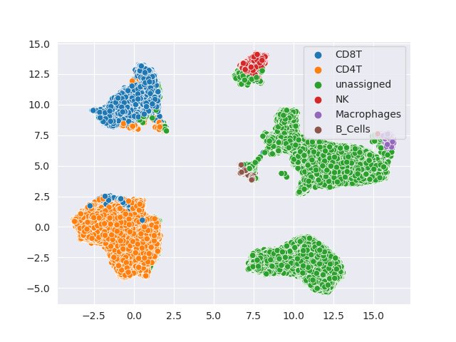
Much better!
DR Evaluation
Have you wondered which DR method is the best? Well, you can benchmark it yourself! This comes in two steps! First, you will need to choose metrics and evaluate your DR methods! Then, you can rank your methods according to these methods!
Currently, we do not support using custom methods for this framework. However, we have the following categories of metrics:
Global Structure Preservation (“global”)
Local Structure Preservation (“local”)
Downstream Performance (“downstream”)
Concordance (“concordance”)
Note
The concordance category is more advanced! We will detail this more in the tutorial section.
Simple Evaluation with Auto Clustering
For DR evaluation, we need clustering labels for both the original data and all the DR embeddings.
We offer a builtin pipeline with KMeans clustering for you to evaluate your dimension reduction
in one simple step!
>>> results.evaluate(category = ["global", "local", "downstream"], auto_cluster = True, n_clusters = 20)
Evaluating global...
Evaluating local...
Evaluating downstream...
Note
We do recommend you change n_clusters according your knowledge of your dataset. If you have a rough
idea of the types of cells present, it is a good idea to use that to your advantage.
With this, you have obtained your first DR evaluation! To check the results, simply access the evaluations
attribute, which is a dictionary:
>>> results.evaluations
{'global': {'spearman': {'PCA': 0.5525689817179995, 'UMAP': 0.2008244633670485, 'open_tsne': 0.39277360696372215},
 'emd': {'PCA': 2.2033917947258224, 'UMAP': 3.112385214988549, 'open_tsne': 27.49076176658772}},
 'local': {'knn': {'PCA': 0.0005694575510071263, 'UMAP': 0.0023624353258924215, 'open_tsne': 0.0044678012430444825},
 'npe': {'PCA': 1488.405, 'UMAP': 997.0799999999999, 'open_tsne': 1180.4850000000001}},
 'downstream': {'cluster reconstruction: silhouette': {'PCA': 0.06870182580853562, 'UMAP': 0.30413094, 'open_tsne': 0.25822831903485394},
 'cluster reconstruction: DBI': {'PCA': 2.790046489762818, 'UMAP': 1.8574548809614353, 'open_tsne': 1.3668004451334124},
 'cluster reconstruction: CHI': {'PCA': 90455.42338884463, 'UMAP': 138076.51781759382, 'open_tsne': 68364.87227338477},
 'cluster reconstruction: RF': {'PCA': 0.5735979292493529, 'UMAP': 0.888894367065204, 'open_tsne': 0.8947121903118452},
 'cluster concordance: ARI': {'PCA': 0.36516898619341764, 'UMAP': 0.6103950568737259, 'open_tsne': 0.5267480266406396},
 'cluster concordance: NMI': {'PCA': 0.6099045072502076, 'UMAP': 0.7625670100165506, 'open_tsne': 0.7245013680103589},
 'cell type-clustering concordance: ARI': {}, 'cell type-clustering concordance: NMI': {}}}
This is a nested dictionary with the following levels:
Categories
Metrics/Sub-categories
Embedding Names
This can be a little confusing, but you can access the sub-levels individually:
>>> results.evaluations["global"]
{'spearman': {'PCA': 0.5525689817179995, 'UMAP': 0.2008244633670485, 'open_tsne': 0.39277360696372215},
 'emd': {'PCA': 2.2033917947258224, 'UMAP': 3.112385214988549, 'open_tsne': 27.49076176658772}}
or you can look at individual metrics:
>>> results.evaluations["global"]["emd"]
{'PCA': 2.2033917947258224, 'UMAP': 3.112385214988549, 'open_tsne': 27.49076176658772}
If you are so inclined, you can utilize these results directly. However, if you would like us to do the work for you, read on!
Note
Notice that there are no values for cell type-clustering concordance: ARI and cell type-clustering concordance: NMI.
This is because we don’t have a builtin pipeline for cell typing. You must provide these information on your own, which is
covered in the next section.
Use Your Own Labels
If you are a more advanced user, you may be aware that KMeans may not be the ideal solution for CyTOF.
You may wish to cluster using FlowSOM in R or your own custom toolchain. If you have these data, you
can easily add them to the object and them perform evaluations as usual:
>>> results.add_evaluation_metadata(original_labels = original_labels,
...                                 embedding_labels = embedding_labels)
These are the bare-minimum needed! Here, original_labels is a numpy array. On the other hand,
embedding_labels is a dictionary with name of DR methods as keys and numpy arrays
of labels as the values. You can, of course, load these data using the methods demonstrated above!
However, if you also have cell types:
>>> results.add_evaluation_metadata(original_labels = original_labels,
...                                 original_cell_types = original_cell_types,
...                                 embedding_labels = embedding_labels,
...                                 embedding_cell_types = embedding_cell_types)
which will allow you to run Cell Type-Clustering Concordace metrics as part of the downstream category. Here,
original_cell_types is just a numpy array, whereas embedding_cell_types is a dictionary.
Afterwards, you can run your DR evaluation as usual using the “Simple” method. All the downstream toolchains
remain the same, except that the auto_cluster and n_clusters parameters no longer play a role:
>>> results.evaluate(category = ["global", "local", "downstream"])
Evaluating global...
Evaluating local...
Evaluating downstream...
Rank DR Methods
Now, you can finally rank your methods! This will be fairly easy:
>>> results.rank_dr_methods()
{'PCA': 1.7083333333333333, 'UMAP': 2.25, 'open_tsne': 2.0416666666666665}
As you can see, this returns a dictonary with method names the methods as keys and their scores as values. If you see decimals, don’t panic! at your computer! We rank each metric individually and the final results are appropriately weighted! Here, larger score is better! Obviously, if you have read our paper, you know that UMAP is pretty good at what it does when compared to PCA and tSNE!
If you desire to use your own metrics and use our ranking methods, be sure to read Custom DR Evaluations tutorial for details on how you can do so.
Save Your Results
After running your DR and evaluations, you will likely want to save your results since you don’t necessarily want to run these methods again, especially if they’re trivially fast to run. We offer a few methods to quickly save your results.
To save your embeddings, you can simply run:
>>> results.save_all_reductions(save_dir="YOUR_DIR_PATH", delimiter=",")
This automatically save all your embeddings into your specified directory in plain text files. And of course, you can customize it a little by changing the delimiter, whether to overwrite existing files, etc. To save your evaluation results, you can call a simple method as well:
>>> results.save_evaluations(path="YOUR_FILE_PATH")
Note, here the path is the full path, not the directory. The results will be saved
as a csv file.
Pipeline At a Glance
Putting everything together, we will have a pipeline like this:
>>> from CytofDR import dr
>>> results = dr.run_dr_methods(expression, methods=["umap", "open_tsne", "pca"])
>>> results.evaluate(category = ["global", "local", "downstream"])
>>> results.rank_dr_methods()
Or alternatively with your own clusters and cell types:
>>> from CytofDR import dr
>>> results = dr.run_dr_methods(expression, methods=["umap", "open_tsne", "pca"])
>>> results.add_evaluation_metadata(original_labels = original_labels,
...                                 original_cell_types = original_cell_types,
...                                 embedding_labels = embedding_labels,
...                                 embedding_cell_types = embedding_cell_types)
>>> results.evaluate(category = ["global", "local", "downstream"])
>>> results.rank_dr_methods()
Congratulations! You’ve made it through the quickstart guide! Give yourself a high five and start performing DR! For more detailed documentations, look around on this website!
What Next?
For further reading, head to the Tutorial section. Here are a few tips:
If you’re interested in preprocessing and further IO options, visit IO and Preprocessing with PyCytoData.
Go look at DR Metrhods and Usage and find out how you can customize your DR methods.
Read up on our Evaluation Metrics to know more about our framework!
Be sure to check out the References as well as Our Paper!